5 Game-changing Excel Formulas

In a normal day as an SEM analyst I will be working in Microsoft Excel for at least a couple of hours, doing tasks ranging from data analysis, to reports, to writing Search Network ads on a large scale. When this much of your day is spent working in one program it is nice to learn the little tricks that can help expedite and simplify things. I am going to break down several Excel formulas that can help you on a daily basis.

1. =LEN()

When I am creating and writing ad copy for large accounts, I like to use Microsoft Excel so it can be easily uploaded through Google AdWords Editor. One of the difficulties in writing ad copy for search engines is the strict character limit. The function “=len()” is a simple function that tells you how many characters, including spaces, are included in a selected cell. Simply put the name of the cell you are interested in inside the parentheses and Excel will return a number.

2. =CONCATENATE()

Concatenate is a function that connects several strings of text together. This can either be done through text that you manually type into the equation or it can grab text out of a desired cell. It can be used for a variety of information. In the example provided below, the city and state columns are combined, creating the location column using the formula =CONCATENATE(B4,”, “,C4).

3. =VLOOKUP()

The vertical lookup formula (VLOOKUP) is one of the most useful Excel tools. It looks for a value in the leftmost column of a table and then returns a value in the same row from the column you specify. This sounds pretty complex, but once you see it used it becomes clear how valuable it is. For example let’s say you have the two following tables of data:

For reporting purposes you want these two tables to be combined, and while you could copy and paste the data where it matches, it’s really not a scalable plan. By using the formula =VLOOKUP(B4,$M$3:$O$6,2,FALSE), you can quickly create the following table:

4. =IF()

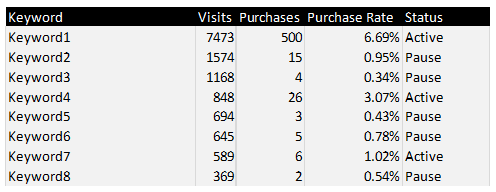
If statements might be the second most valuable Excel formula there is. It allows you to check the value or text in a desired cell and return a different answer or phrase depending on whether the selected cell meets or fails to meet your given criteria. For example, if you have a list of keywords and you want to pause all of the keywords that have a conversion rate below 1%, then you can use the following formula to split your list into the categories of “Pause” and “Active”: =IF(F4<0.01,”Pause”,”Active”)

5. =LEFT/RIGHT ()

The last formula I’m going to describe is =LEFT() and =RIGHT(). These formulas are essentially the opposite of the =CONCATENATE() formula. Each takes a selected string of text and returns a specified amount of characters starting on either the leftmost or rightmost character of the word. This can be helpful when you need to separate an input that is combined in a column like the example below where we are splitting City and Zip Code into just Zip Codes, using this formula =RIGHT(B4,5).

I hope these formulas help you the next time you are in Excel. They may seem tough at first, but once you use them a couple of times they will become second nature. If you ever have any questions about how these or any Excel formulas work, you can just click the button located next to the formula bar.

Are there some other Excel formulas or shortcuts you’d like to learn? Leave us a comment in the section below, email us at info@perfectsearchmedia.com, or tweet us @Perfect_Search!